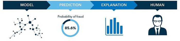
MEDICAL FRAUD DETECTION- An End to End ML Case Study
To predict the potentially fraudulent providers based on the claims filled by them

Companies fighting medical claim fraud, have a tough task of telling fraudulent claims from honest ones. Although majority of claimants submit honest and accurate claims, a small fraction gives in to the financial incentive and exaggerates the complexity and size of the claim
For example : I am the only one in my family with health insurance, but I let my brother and cousin use my card to receive health care benefits. This is a fraud to claim medical benefits.
Let me take another instance: My medical records were falsified by a physician’s assistant to support the billing of insurance programs for procedures that were never performed. So basically, for services that weren’t taken by me, false billing was made to claim the amount.
How do we know whether the services billed were actually performed? Is the actual patient listed and whether the eligibility is verified? Incorrect reporting of diagnoses or procedures …Or What?
We’ll get to know the answers to these questions soon. We will deep dive to figure out the potentially fraudulent providers based on the claims filed by them. Lets Get Started folks!!👊
TABLE OF CONTENTS :
- Understanding the Given Problem Statement
— 1.1 Business Problem
— 1.2 Business Objectives and Constraints
— 1.3 Source of Data and Dataset Description
— 1.4 ML Problem Formulation
— 1.5 Performance Metrics
2. Exploratory Data Analysis
— Univariate and Bivariate Analysis:
— 2.1 Physician/Provider/Beneficiary Analysis
— 2.2 Age and Gender Analysis of Beneficiary
— 2.3 The number of days it took to get the claim
— 2.4 Hospitalization days
— 2.5 Race/State/Country
— 2.6 Claim Amount
— 2.7 Diagnosis and Procedure Codes
— 2.8 Conclusions from EDA
3. Feature Engineering
4. ML Algorithms
— 4.1 Decision Tree Classifier
— 4.2 Xgboost Classifier
—4.3 Stacking Classifier
— 4.4 Custom Ensemble Implementation
5.Model Deployment
— 5.1 Flask API
— 5.2 Further improvements
— 5.3 References
UNDERSTANDING THE GIVEN PROBLEM STATEMENT
BUSINESS PROBLEM
Healthcare is important in the lives of many citizens, but unfortunately the high costs of health-related services leave many patients with limited medical care. There are a number of issues facing healthcare and medical insurance systems, such as a growing population or bad actors (i.e. fraudulent or potentially fraudulent physicians/providers). Here , we focus our attention on fraud. The detection of fraud within healthcare is primarily found through manual effort by auditors or investigators searching through numerous records to find possibly suspicious or fraudulent behaviours.

Now there may be a lot of instances where people may try to play a foul game to extract big amounts. Insurers need to detect unethical medical billing practices early to reduce claim leakage and process legitimate bills faster.
BUSINESS OBJECTIVES AND CONSTRAINTS
Now that the Business Problem is clear , we need to identify the associated business objectives and constraints. This is the most important part before moving forward to formulating the Machine Learning Problem, as they would define the kind of solution that we would need to develop.
Objectives:
- The goal of this project is to “ predict the potentially fraudulent providers” based on the claims filed by them.
- Along with this, we will also discover important variables helpful in detecting the behaviour of potentially fraud providers. Further, we will study fraudulent patterns in the provider’s claims to understand the future behaviour of providers.
Constraints:
- Model Interpretability is very important for predicting a Potential Fraud or not.
- No strict Latency requirements, as the objective is more about making the right decision rather than a quick decision. It would be fine and acceptable if the model takes few seconds to make a prediction.
- Misclassification could prove very costly. We do not want the model to miss out on claims which are actually fraud.
SOURCE OF DATA
The data has been taken from the following kaggle link:
DATASET DESCRIPTION
- Inpatient Data and Outpatient Data:
- BeneID : A Unique Id for the beneficiary seeking claim
- ClaimID : A Unique Id for the claim submitted for reimbursement
- ClaimStartDt / ClaimEndDt : It marks the start of claim submission and end of claim settlement
- Provider : A unique Id for claim providers
- InscClaimAmtReimbursed : Amount reimbursed to patient
- AttendingPhysician : Id for physicians who physically attended patients
- OperatingPhysician/OtherPhysician: Id for physicians who operated on patients or performed other operations
- AdmissionDt / DischargeDt : It marks the date on which patient got hospitalized and discharged respectively
- ClmDiagnosisCode : Diagnosis codes undergone by patients
- ClmProcedureCode : Procedure codes undergone by patients
2. Beneficiary Data :
- BeneID : A Unique Id for the beneficiary seeking claim
- DOB/DOD : Date of Birth/Death for beneficiaries seeking claim
- Gender/Race/State/Country : Details of the beneficiaries seeking claim
- Comorbid Related Details : ChronicCond_Alzheimer,RenalDiseaseIndicator,ChronicCond_Depression,ChronicCond_Cancer etc. related details of patients
- Reimbursed/Deductible Amounts: Amount to be reimbursed or the actually paid amount
3. Label data:
- Provider: A unique Id for claim providers
- Potential Fraud: Yes and No indicate whether the provider is potentially fraud or not
ML PROBLEM FORMULATION
We can now formulate the machine learning problem statement, which would adhere to those objectives and constraints.
- We can identify that it is a Supervised Learning Classification problem, which contains the training data points along with their Class Labels. Here the Class Labels represent whether a given claim is Potentially Fraud or not.
- We also realize that it is a Binary Classification problem, that is it contains just 2 classes, Yes and No to indicate whether the provider is potentially fraud or not
- There is an imbalance in my class labels(38.1% to 61.9%)
Once we have built the final Machine Learning Model, we can then deploy it to instantly check whether a given claim is Fraud or Not.
PERFORMANCE METRICS
Macro F1 Score: According to the documentation of Sklearn,
'macro': Calculate metrics for each label, and find their unweighted mean. This does not take label imbalance into account.This means that:
There is an imbalance in my class labels(38.1% to 61.9%).A macro f1 score gives equal weightage/importance to each class.
We use macro-averaging to weight our metric towards the smallest one(class imbalance).This metric is insensitive to the imbalance of the classes and treats them all as equal.2. AUC ROC Score: Due to probabilistic scores, AUC helps us identify how well the model is able to distinguish between target labels especially when the target label is probabilistic value.
EXPLORATORY DATA ANALYSIS
Exploratory Data Analysis is a vital step in a data science project. The main pillars of EDA are data cleaning, data preparation, data exploration, and data visualization.
So to begin with, let us perform the merge operation of our csv files to formulate the patient_data
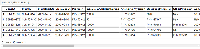
Computing the percentage missing values for each column in our data
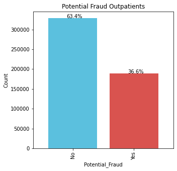
Beginning with a simple bar plot to find out the proportion of labels i.e. Potential Fraud being Yes/No(Binary Classification)


For inpatients, the frauds are occuring sligtly more.
There are 53.6% Frauds and 46.4% Non Frauds.
For outpatients, the number of frauds are less.
There are 36.6% Frauds and 63.4% Non Frauds.
A simple reasoning to these could be the fact that outpatients are not admitted, hence they don’t commit frauds. On the other hand inpatients are admitted hence they might want to retrieve more money.
PHYSICIAN ANALYSIS
So now I’ll analyze how physicians who have attended/operated on more/less patients could play a vital role in fraud detection


Top 5 physicians with most attended cases for Outpatients;
PHY330576 2534
PHY350277 1628
PHY412132 1321
PHY423534 1223
PHY314027 1200

Top 5 physicians with most attended cases for Inpatients;
PHY422134 386
PHY341560 274
PHY315112 208
PHY411541 198
PHY431177 195The physicians who have attended more patients are likely doing more frauds as evident from countplots. It is a no-brainer that this feature ‘physician_count’ could be a very crucial one. Secondly the above countplots clearly show that physicians with maximum attended cases are likely to commit frauds.
A similar analysis is done on the OperatingPhysician , OtherPhysician and Beneficiaries
PROVIDER ANALYSIS


Top 5 providers with most provided services for Outpatients;
PRV51459 8240
PRV53797 4739
PRV51574 4444
PRV53918 3588
PRV54895 3433

Top 5 providers with most provided services for Inpatients;
PRV52019 516
PRV55462 386
PRV54367 322
PRV53706 282
PRV55209 275
Analysis using a Pointplot


Age and gender analysis of beneficiary

Now here I’ll group the ages in intervals of 10
Then doing a Bivariate Analysis to reach to certain conclusions
Gender        1     2
age_group
(30, 40]    413   375
(40, 50]    826   821
(50, 60]   1324  1372
(60, 70]   4083  4908
(70, 80]   5944  7619
(80, 90]   3762  6136
(90, 100]   698  1874
Gender         1       2
age_group
(30, 40]    5370    5254
(40, 50]   10134   10740
(50, 60]   16318   17759
(60, 70]   53829   66316
(70, 80]   77220  100639
(80, 90]   45088   75230
(90, 100]   8085   21735
PotentialFraud    No   Yes
age_group
(30, 40]         340   448
(40, 50]         691   956
(50, 60]        1115  1581
(60, 70]        3819  5172
(70, 80]        5642  7921
(80, 90]        4234  5664
(90, 100]       1077  1495
PotentialFraud      No    Yes
agegrp
(30, 40]          6828   3796
(40, 50]         13375   7499
(50, 60]         22030  12047
(60, 70]         76394  43751
(70, 80]        112710  65149
(80, 90]         75902  44416
(90, 100]        18585  11235
A simple takeaway from my ‘age & gender’ analysis is that:
More/Less age is not a parameter to decide whether a fraud is likely to be commmitted or not
Our grouped bar plots show that:
70–80 age group is commonly found.
Within 70–80 age group, more frauds happen for inpatients whereas less frauds for outpatients.
NUMBER OF DAYS IT TOOK TO GET THE CLAIM FOR OUTPATIENTS AND INPATIENTS


The plots indicate that:
1. ClaimDays_count could be a very crucial feature as:
-> For outpatients, top 5 days it took and the count of beneficiaries who got it it that duration
Days Frequency of occurence
1 453348
21 24312
2 11960
3 4366
15 2735
-> For inpatients, top 5 days it took and the count of beneficiaries who got it it that duration
Days Frequency of occurrence
4 6899
3 6119
5 4993
2 4599
6 3579
-> From the outpatients countplot it is evident that majority claims just took 1 day. Most of these were non frauds.
-> From inpatients countplot it is evident that most claims took an average of 4 to 9 days with some of them being frauds and rest non frauds.
Analysis on Race, State, Country

Majority patients belong to race 1
Among Patients belonging to race 1,around 30k have not committed frauds and about 17k have committed frauds.
So ‘race’ could be an important feature.

Top 5 states where people have submitted more claims are: States with codes {5,10,33,45,14}
So in my countplot it is evident that state 5 is more likely to have more fraud claims.

Top 5 countries where people have submitted more claim requests are:
Countries with codes {200,10,20,470,60}
ANALYSIS ON CLAIM_AMOUNT
Here is a kernel density estimation plot for a visual look


Plots indicate that:
For Inpatients, a higher amount is reimbursed compared to outpatients.
The reasoning being the fact that inpatients seek more claim due to their hospital expenditure.
Let us group the amounts reimbursed into intervals now
For outpatients the intervals are in a lesser range because of the amount being less and vice versa for inpatients

PotentialFraud      No    Yes
amountgrp
(0, 50]         107411  61838
(50, 100]       103799  60252
(100, 200]       26885  15297
(200, 400]       27964  16285
(400, 600]       14623   8268
(600, 800]        7433   4470
(800, 1000]       4870   2783
(1000, 1500]      6699   3920
(1500, 2000]      5606   3281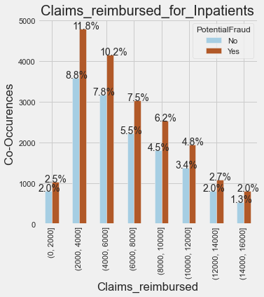
PotentialFraud    No   Yes
amountgrp
(0, 2000]        805  1032
(2000, 4000]    3578  4786
(4000, 6000]    3173  4144
(6000, 8000]    2225  3036
(8000, 10000]   1811  2525
(10000, 12000]  1377  1942
(12000, 14000]   813  1083
(14000, 16000]   532   806
It is evident that:
> The majority claims remibursed are in range 2000 to 4000.
-> Claims from 2000 to 12000 are reimbursed quite often.
-> More fraud claims are done here in inpatients.
We can conclude from here that:
If the InscClaimAmtReimbursed is less then it is less likely a fraud
On the other hand if the amount is more, then chances of fraud increase, though there is an overlap.
PROCEDURE CODES AND DIAGNOSIS CODES ANALYSIS

- Top 10 Diagnosis codes with their frequency of occurence are:
Code Frequency
4019     77056
25000    37356
2724     35763
V5869    24904
4011     23773
42731    20138
V5861    20001
2720     18268
2449     17600
4280     15507
- Top 10 Procedure codes with their frequency of occurence are:
Code Frequency
4019.0    1959
9904.0    1152
2724.0    1054
8154.0    1022
66.0       901
3893.0     854
3995.0     809
4516.0     651
3722.0     589
8151.0     463
CONCLUSIONS FROM EDA
From the Exploratory Data Analysis, the following observations were made: -
-> There are less fraud claims in my data comapared to non fraud claims. 212796 Frauds and 345415 Non Frauds. For inpatients, the frauds are occurring slightly more. Whereas for outpatients they are less in number.
-> Physicians who have attended more patients are more likely to commit fraud. The physicians with ids PHY422134,PHY341560,PHY315112,PHY411541,PHY431177} have attended the most patients(inpatients).
-> The physicians with ids{PHY330576,PHY350277,PHY412132,PHY423534,PHY314027} have attended the most patients(outpatients).
-> Operating_physician_count could also be a very crucial feature as the physicians who have operated on more patients are likely doing more frauds.
Top 5 physicians with most operated cases for Inpatients;{PHY429430,PHY341560,PHY411541,PHY352941,PHY314410}
Top 5 physicians with most operated cases for Outpatients;{PHY330576,PHY424897,PHY314027,PHY423534,PHY357120}
-> There is a clear demarcation in determining the fact that top 20 providers whether for inpatients or outpatients have all commited frauds.
-> Unlike the provider or physician count, here there is no substancial clarity as to whether a beneficiary with more claims taken has done a fraud.This means this(Benef_count) is not a very good feature but surely will play some role.
-> For beneficiaries(Inpatients) who have seeked more claims or have a higher count, are more likely to commit frauds.
For beneficiaries(Outpatients) who have seeked more claims or have a higher count, there is no substaincial information to conclude anything.
-> ‘Age’ is not a useful feature considering the fact that no visible conclusions can be drawn from the boxplots. More/Less age is not a parameter to decide whether a fraud is likely to be commmited or not.
-> For outpatients it is evident that mojority claims just took 1 day. Most of these were non frauds. From inpatients countplot it is evident that most claims took an average of 4 to 9 days with some of them being frauds and rest non frauds.
-> Majority patients belong to race 1. Among Patients belonging to race 1,around 30k have not commited frauds and about 17k have commited frauds. So ‘race’ could be an important feature.
-> Top 5 states where people have submitted more claims are: States with codes {5,10,33,45,14} .So it is evident that state 5 is more likely to have more fraud claims.
-> For Inpatients, a higher amount is reimbursed compared to outpatients. The reasoning being the fact that inpatients seek more claim due to their hospital expenditure.
-> The top 5 Procedure Codes are {4019.0,9904.0,2724.0,8154.0,66.0} and top 5 Diagnosis Codes are {4019,25000,2724,V5869,4011}.
FEATURE ENGINEERING
Do you know that data scientists spend around 80% of their time in data preparation?
Feature engineering is a vital part of this. Without this step, the accuracy of a machine learning algorithm reduces significantly. A typical problem solving starts with data collection and exploratory analysis. Data cleaning comes next. Each column is a feature. But these features may not produce the best results from the algorithm. Modifying, deleting and combining these features results in a new set that is more adept at training the algorithm.
Feature engineering in machine learning is more than selecting the appropriate features and transforming them.
Not only does feature engineering prepare the dataset to be compatible with the algorithm, but it also improves the performance of the machine learning models.
Feature Engineering includes things like imputation(filling missing or nan values),handling outliers, grouping operation, feature split, binning etc.

- A feature ‘is_beneficiary_present’ is not required as %age null values are 0 meaning it is always present.
- A feature ‘is_operating_physician_present’ makes sense as there are 79% null values here.
The output from feature engineering is fed to the predictive models, and the results are cross-validated.
Feature ‘whether_admitted’:: For inpatients the value will be 1 and for outpatients it will be 0
Features ‘is_dead’ and ‘is_alive’:: For patients with Date_of_Death as NaN,it is 0, else 1
%age null values in date_of_death column are 99.25%, so I’ll include ‘is_dead’ as a feature -> wherever ‘nan’ is present, it may mean that either the person is alive or the data is missing. I’ll replace a non null value with 1 meaning the person is dead. Else with 0.
I’ll include ‘is_alive’ as a feature based on the fact that if dod column has non null values, means he is not alive.(equal to 0) else 1.
Now I’ll add some features which showed a clearer picture is capturing whether a claim is fraud or not in my EDA analysis
Count of physicians/beneficiary/provider
- Feature ‘operate_physician_count’ It implies,the number of times a physician operated.In my EDA analysis, it was evident that if the count is more then it might be a potential fraud
- Feature ‘attendphysician_count’:: It implies, the number of times a physician attended a patient. In my EDA analysis, it was evident that if the count is more then it might be a potential fraud
- Feature ‘BeneID_count’:: It implies,the number of times a beneficiary submitted claims. In my EDA analysis, it was evident that if the count is more then it might be a potential fraud. Though a clear demarcation as in physician_count was not obtained here in my EDA.
- Feature ‘provider_count’:: It implies,the number of times a provider gave services.In my EDA analysis, it was evident that if the count is more then it might be a potential fraud. And a clear demarcation was obtained here in my EDA which shows it is a useful feature
Feature ‘Claim_days’:: It implies, the number of days it took for a claim to be reimbursed. In my EDA analysis, it was evident that if the days are more then it might be a potential fraud, though it was not necessary.
Feature ‘hospitalization_days’:: It implies, the number of days patient was admitted. In my EDA analysis, it was evident that if the days are more then it is a potential fraud.
Feature ‘total_diff_amount’:: Firstly I’ll sum the i/p and o/p reimbursement amounts, then i/p and o/p deductible amounts. Finally the total_diff_amount will be the difference of the two.
Now I’ll include the top 7 diagnosis codes and 7 procedure codes as my 14 new features with a 0/1 value.
I’ll add 3 new features: is_primary,is_secondary,is_tertiary:: They actually serve the purpose of filling ‘nan’ value i.e. imputation. the nan values in ‘AttendingPhysician,OperatingPhysician,OtherPhysician’ get replaced by 0/1 in these features
Replace the yes/no in PotentialFraud column with 1/0, y/0 in RenalDiseaseIndicator with 1/0
Adding 6 new features which indicate the count of top 3 diagnosis and procedure codes
Dropping other columns and finalizing the data
Data Normalization
Attributes are often normalized to lie in a fixed range — usually from zero to one — by dividing all values by the maximum value encountered or by subtracting the minimum value and dividing by the range between the maximum and minimum values.
ML Algorithms
Now we have reached that stage where we have a well organized and featured dataset to work upon. So we’ll experiment with machine learning techniques like decision trees, xgboost, stacking clsssifier and finally a custom ensemble implementation. I’ll tell you why isn’t a stacking classifier used in real world.
You’ll get to know which model performs the best on this data.

DecisonTreeClassifier|| Hyperparameter Tuning
Decision trees are a method for classifying subjects into known groups. They’re a form of supervised learning.
The clustering algorithms can be further classified into “eager learners,” as they first build a classification model on the training data set and then actually classify the test dataset. This nature of decision trees to learn and become eager to classify unseen observations is the reason why they are called “eager learners.”

XGBoostClassifier|| Hyperparameter Tuning
XGBoost has become a widely used and really popular tool among Kaggle competitors and Data Scientists in industry, as it has been battle tested for production on large-scale problems. It is a highly flexible and versatile tool that can work through most regression, classification and ranking problems as well as user-built objective functions. As an open-source software, it is easily accessible and it may be used through different platforms and interfaces.
The algorithm was developed to efficiently reduce computing time and allocate an optimal usage of memory resources. Important features of implementation include handling of missing values (Sparse Aware), Block Structure to support parallelization in tree construction and the ability to fit and boost on new data added to a trained model

STACKING CLASSIFIER
Stacking is a supervised ensemble learning technique. The idea is to combine base predictive models into a higher-level model with lower bias and variance.
Stacking lacks interpretability. After x layers of stacked models, finding the contribution of a given input to final prediction accuracy becomes a full-time job. That is why in real world, where reasoning to a prediction is required,this is not used
CUSTOM ENSEMBLE MODEL
1) Split your whole data into train and test(80–20)
2) Now in the 80% train set, split the train set into D1 and D2.(50–50).
Now from this D1 do sampling with replacement to create d1,d2,d3….dk(k samples).
Now create ‘k’ models and train each of these models with each of these k samples.
3) Now pass the D2 set to each of these k models, now you will get k predictions for D2, from each of these models.
4) Now using these k predictions create a new dataset, and for D2, you already know it’s corresponding target values, so now you train a meta model with these k predictions.
5) Now for model evaluation, you have can use the 20% data that you have kept as the test set. Pass that test set to each of the base models and you will get ‘k’ predictions. Now you create a new dataset with these k predictions and pass it to your metamodel and you will get the final prediction. Now using this final prediction as well as the targets for the test set, you can calculate the models performance score.
Now for the best model i.e. xgboost we could go with the approach of finding the probabilistic output and then using the best threshold making the final prediction. Here’s a glimpse of that
SUMMARIZING
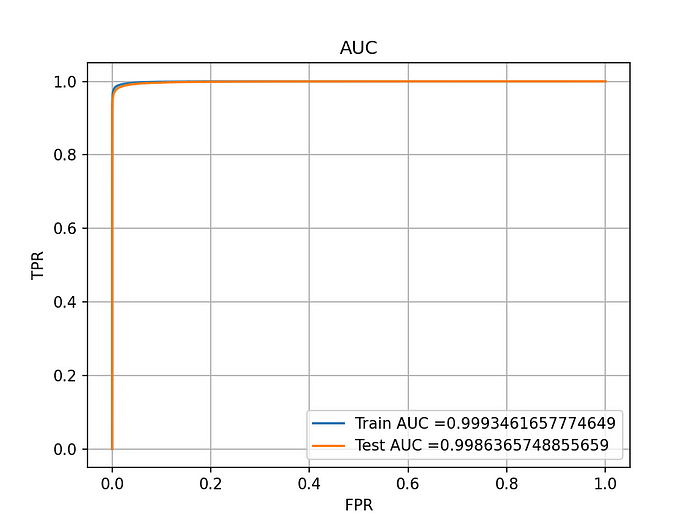
So we summarize the results of our 4 models that we compared. Xgboost performed reasonably well with a score above 0.99. It gives us interpretable results which was one of the main business constraints of our task.
Here is a complete pipeline for whatever we did till now. From feature engineering all the way till predictions being made on our test data
MODEL DEPLOYMENT
We tend to forget our main goal, which is to extract real value from the model predictions.
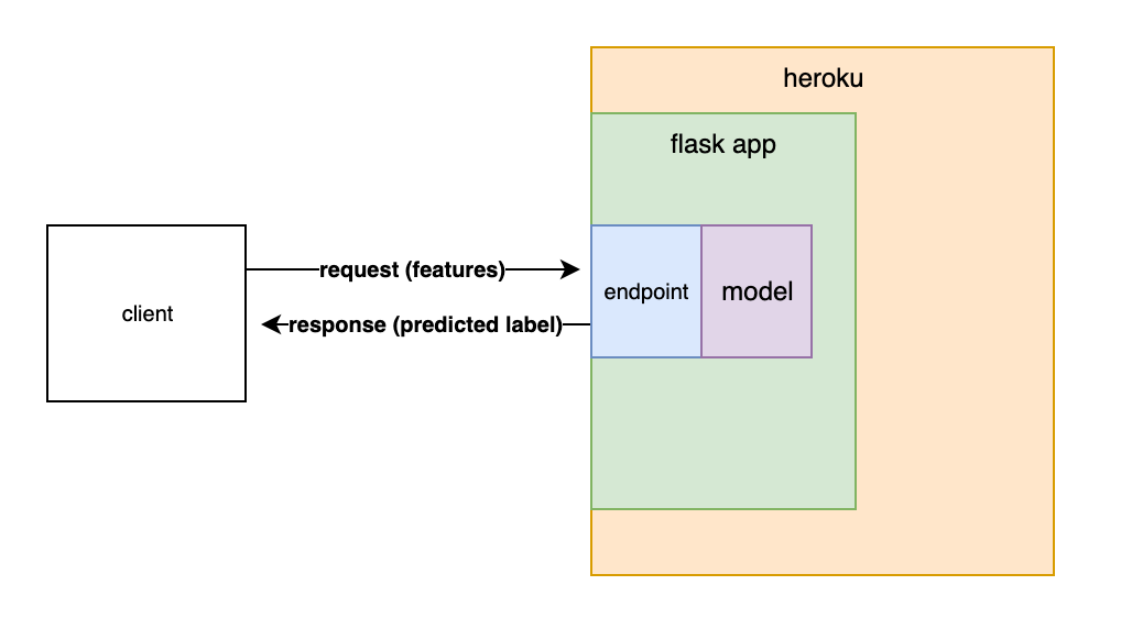
Deployment of machine learning models or putting models into production means making your models available to the end users or systems. However, there is complexity in the deployment of machine learning models. Here I used the Flask API to deploy my model in my local system.

Here’s a video showing the deployed model and its working
FURTHER IMPROVEMENTS
Deep learning Techniques will further add improvements in determining the fraud claims
Improvements in this domain will help in detecting a series of fraud physicians, providers and beneficiaries
It will help in improving the state of economy by reducing inflation caused by fraud people and lowering down insurance premiums which will not cause health to become more costlier
Github Profile:
https://github.com/PranjalDureja0002/Health_Fraud
LinkedIn Profile:
https://www.linkedin.com/in/pranjal-dureja-89409a1a5/
REFERENCES
Data Obtained: https://www.kaggle.com/rohitrox/healthcare-provider-fraud-detection-analysis/discussion/101993
